Physics-Grounded ML for Adaptive Biomedical Sensing: Three Complementary Paths
TL;DR — When sensor data is sparse, noisy, or expensive to acquire, physics-grounded machine learning offers three complementary strategies: (1) physics-informed neural networks that penalize PDE residuals to regularize reconstruction, (2) energy-based models that maintain posterior beliefs to drive adaptive measurement selection, and (3) solver-coupled networks that embed conventional numerical solvers directly into training. We sketch how these three threads converge into a unified vision for autonomous experimental systems in biomedical sensing.
The Problem: Data Scarcity in Biomedical Sensing
Modern biomedical sensing — whether mmWave radar for contactless health monitoring, sparse-angle CT for low-dose imaging, or adaptive microscopy for live-cell observation — face a common constraint: we never have enough data. Sensors are sparse (few measurement points), noisy (low signal-to-noise ratio), or expensive (radiation dose, acquisition time, tissue damage). In all three cases, a purely data-driven model risks overfitting the limited observations and hallucinating unphysical structure in unobserved regions.
The core research question is: How do we reconstruct and reason about physical fields when observations are fundamentally incomplete?
This post explores three complementary approaches we have been prototyping, each addressing a different facet of the problem. Together, they point toward a unified framework for physically-grounded, uncertainty-aware, adaptive experimental design.
Thread 1: Physics as Regularizer — PINNs for Sparse Sensing
The Setup
In our first toy problem, we simulate a 1D mmWave-inspired wave field governed by a Helmholtz-style equation:
u_xx(x) + k(x)^2 u(x) = s(x), x ∈ [0, 1]with a piecewise coefficient k(x) (simulating a material interface), a localized Gaussian source s(x), and Dirichlet boundary conditions. Only 20 sparse, noisy sensors sample the field. The task: reconstruct the full field from these 20 noisy observations.
Baseline vs PINN
We compare two approaches:
- Naive MLP baseline: A standard fully-connected network trained only to minimize MSE on the 20 sensor observations.
- Physics-Informed Neural Network (PINN): The same network architecture, but with additional loss terms penalizing: (a) mismatch at sensor locations, (b) boundary condition violation, and (c) PDE residual at 1200 collocation points across the domain.
Results
| Metric | Baseline MLP | PINN | PINN Advantage |
|---|---|---|---|
| MSE (full field) | 1.86 × 10⁻⁶ | 3.64 × 10⁻⁹ | 510× lower |
| MSE (unsensed regions) | 1.88 × 10⁻⁶ | 3.64 × 10⁻⁹ | 516× lower |
| Relative L₂ error | 12.8% | 0.57% | 23× lower |
| PDE residual norm | 0.297 | 0.023 | 13× lower |
The PINN achieves ~500x lower reconstruction error (1D synthetic Helmholtz problem, 20 sparse noisy sensors) and produces a physically consistent field where the naive baseline interpolates sensor observations with unphysical oscillations. The key insight: when data is sparse, the PDE residual acts as a “free” regularizer that enforces physical consistency in regions where no sensor exists. Note: This result is from a controlled 1D toy problem with known physics. Real-world gains will vary significantly depending on problem dimensionality, noise model, and field complexity.
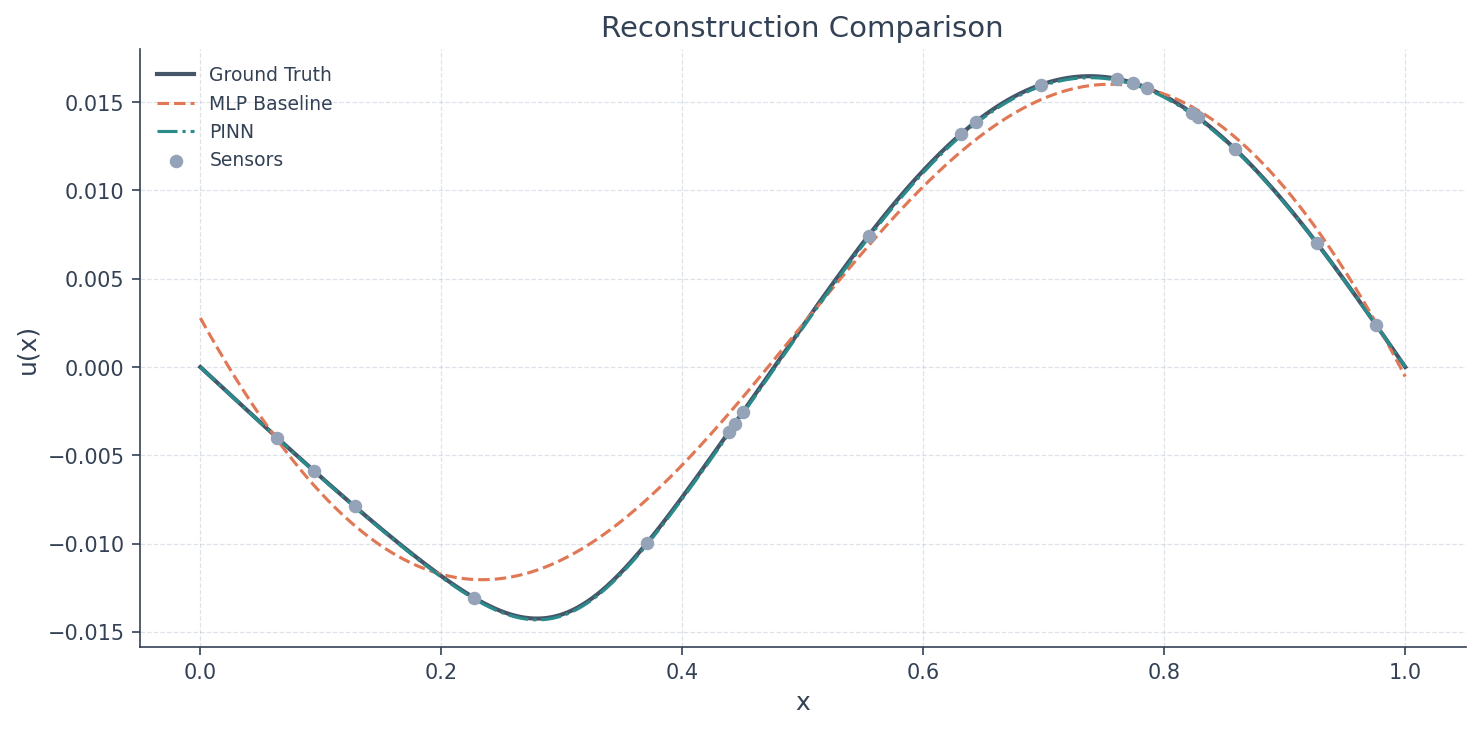 Figure 1: Ground truth (blue), baseline MLP (orange), and PINN (green) reconstructions. The baseline interpolates sparse sensors but violates the wave equation between them; the PINN respects the governing physics everywhere.
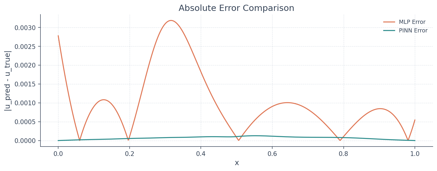 Figure 2: Error fields showing where each model deviates from ground truth. The PINN error is concentrated near the source and interface; the baseline error is distributed across the entire domain.
Limitations
This is explicitly a toy: 1D, synthetic data, known PDE, no real hardware. The PINN convergence is sensitive to loss-weight balance and struggles at higher wavenumbers (k >= 10) without spectral encoding tricks. Nevertheless, the 510× error reduction under sparse/noisy sensing is a clear signal that physics constraints matter.
Thread 2: Uncertainty as Policy — Adaptive Sensing with EBMs
The Setup
In our second toy problem, we flip the perspective: instead of reconstructing a field from fixed sparse sensors, we ask where should the next sensor measurement be taken? The hidden state is a 2D point source location. The measurement device chooses a projection angle and observes a noisy 1D projection. After each measurement, the system must:
- Update its belief about the hidden state
- Estimate uncertainty in that belief
- Choose the next measurement angle to maximize information gain
The Approach: Conditional Energy-Based Models
We use a conditional Energy-Based Model (EBM) to represent the posterior distribution over hidden states given measurement history. The model learns an energy function:
E_θ(x | measurement history)where lower energy means the state x is more plausible given the observations so far. Training uses contrastive divergence with Langevin dynamics sampling. The posterior samples provide both a belief distribution and an uncertainty estimate.
For action selection, we use a simple but principled rule: project the posterior covariance onto each candidate sensing direction and choose the angle with the largest projected variance. If uncertainty is mostly horizontal, measure horizontally; if diagonal, choose a diagonal projection.
The Closed Loop
The full adaptive sensing cycle is:
- Choose initial measurement angle
- Acquire noisy projection
- Update EBM posterior conditioned on new observation
- Sample posterior to estimate uncertainty
- Select next angle based on projected variance
- Repeat until budget exhausted
This is the core of autonomous experimental design: the model doesn’t just passively reconstruct; it actively decides what to measure next.
Limitations
The toy is deliberately restricted: 2D point source, linear forward model, discrete 4-angle action bank, simple variance-based acquisition. The EBM has not yet been runtime-verified in our local workspace. But the structure — physics-based forward model + probabilistic inference + adaptive measurement selection — is the cleanest possible first step toward the full vision.
Thread 3: Solvers as Teachers — NewPINNs
The Setup
Our third thread addresses a fundamental limitation of standard PINNs: loss-weight tuning. In the mmWave PINN, we manually set w_data = 10.0, w_bc = 1.0, w_pde = 1.0. If these weights are misbalanced, the PINN either overfits sensor data (ignoring physics) or oversmooths (ignoring data). Finding good weights is problem-dependent and often requires trial and error.
NewPINNs (Makki et al., 2026, arXiv:2601.17207) propose a radical alternative: remove PDE residuals from the loss entirely. Instead of penalizing residuals, embed a conventional numerical solver (FEM, FVM, or spectral) directly into the training loop and train the network by minimizing solver-consistency. (Note: We have locally reproduced the 1D Burgers benchmark from this preprint — see the “Local Reproduction” subsection below. The 2D benchmarks remain unreproduced in our workspace.)
How It Works
The training loop becomes:
- Network predicts a field
u_pred - Pass
u_predthrough the numerical solver (e.g., NGSolve FEM or FiPy FVM) - The solver advances or corrects the prediction to a physically consistent state
u_solved - Loss = ||u_pred - u_solved||² The network learns to predict fields that the solver barely needs to correct. Physical validity is enforced by construction, not by soft penalty terms.
Benchmarks
The NewPINNs reference implementation includes five benchmarks:
| Benchmark | Dimension | Solver | Network | Target |
|---|---|---|---|---|
| Burgers equation | 1D | Chebfun spectral | Dense | Shock evolution |
| Heat equation | 1D | Chebfun spectral | Dense | Diffusion dynamics |
| ODE inverse | 1D | Numerical | Dense | Parameter recovery |
| Lid-driven cavity | 2D | NGSolve FEM | UNet | Steady Navier-Stokes |
| Fokker-Planck | 2D | FiPy FVM | UNet | Equilibrium density |
The 2D benchmarks are particularly compelling: a UNet predicts velocity/pressure fields, which are then refined by industrial-strength FEM/FVM solvers. This is not a toy; it is a genuine coupling between deep learning and classical numerical analysis.
Local Reproduction: 1D Burgers Head-to-Head
We reproduced the 1D Burgers benchmark (exp-newpinns-003, 2026-07-06) as a direct head-to-head comparison that the original paper does not provide. With identical architecture ([3,64,64,64,64,64,1] tanh MLP), Adam optimizer (lr=1e-3), 4000 iterations, and seed 42:
| Metric | Standard PINN | NewPINN | Advantage |
|---|---|---|---|
| MSE | 3.777 × 10⁻² | 1.618 × 10⁻⁴ | 233× lower |
| Relative L₂ | 4.80 × 10⁻¹ | 3.14 × 10⁻² | 15× lower |
| Training time | 156.7 s | 174.7 s | 1.11× overhead |
NewPINN’s loss dropped below 1e-3 at iteration 175; the standard PINN plateaued at ~0.05 (PDE-residual-dominated) and never reached 1e-3. Error for NewPINN is uniform across time-steps (~1e-4), while PINN error is distributed non-uniformly.
Important caveat from the ablation: A subsequent loss-weight sensitivity sweep (exp-newpinns-005, 2026-07-18, 100 runs over five weight ratios × 10 seeds) refuted the idea that NewPINN eliminates loss-weight tuning. NewPINN is ~6.8× more sensitive to the PDE/data weight ratio than standard PINN, though its best-case accuracy at a tuned weight is 7.6× better. The robustness claim should be read as “loss-weight-tuning-shifted” rather than eliminated — the practitioner still selects the weight, and the cost of a poor choice is higher for NewPINN than for PINN. See the full ablation writeup for details.
This is a single-seed, CPU-only, 1D result on one PDE family (Burgers). On the Helmholtz problem used in Thread 1, NewPINN was MSE-competitive but residual-weak (exp-newpinns-004). The advantage is problem-dependent, not universal.
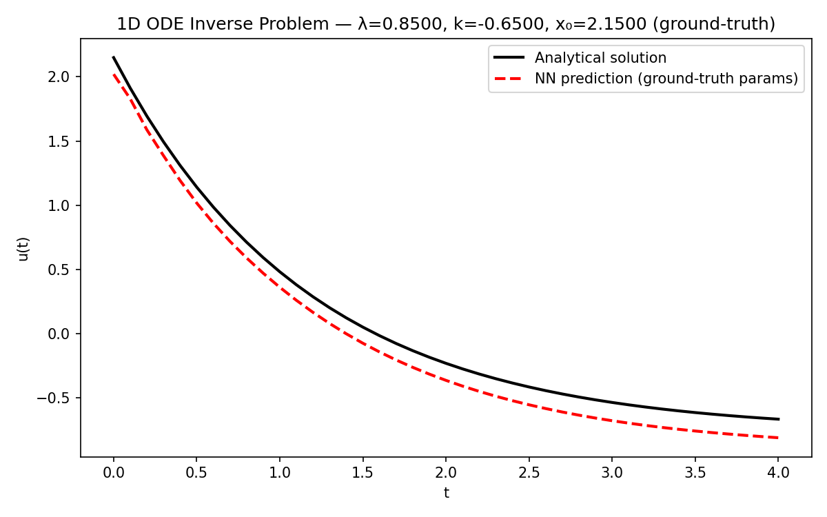 Figure 3: Evaluation result from NewPINNs 1D ODE inverse problem, showing the solver-coupled network’s prediction tracking the reference solution.
Limitations
NewPINNs are computationally expensive: every training step requires running a numerical solver. The 2D benchmarks depend on heavy dependencies (NGSolve, FiPy, PyTorch Lightning) that are not yet installed in our workspace. And the approach assumes the solver is available and trustworthy — a reasonable assumption for well-studied PDEs, but not for novel physics.
Convergence: A Unified Research Vision
How do these three threads fit together? Consider the full pipeline of an autonomous biomedical sensing system:
Sensors → Reconstruction → Uncertainty → Decision → Next Sensors| Stage | Challenge | Our Threads |
|---|---|---|
| Reconstruction | Sparse/noisy data → ill-posed inverse problem | Thread 1 (PINN): Physics regularizes reconstruction; Thread 3 (NewPINN): Solver guarantees physical validity |
| Uncertainty | Point estimates are insufficient for decision-making | Thread 2 (EBM): Posterior samples provide explicit uncertainty |
| Decision | Where to place the next sensor? | Thread 2 (EBM): Variance-based adaptive selection; could be extended with information-theoretic criteria |
| Validation | Is the model actually physical? | Thread 3 (NewPINN): Solver consistency is a hard constraint |
The unified vision is a closed-loop physics-grounded experimental system:
- A NewPINN-style network reconstructs the physical field with solver-guaranteed validity
- An EBM posterior maintains uncertainty over possible field configurations
- An adaptive policy selects measurements to minimize posterior entropy
- A standard PINN serves as a lightweight baseline or pre-training step
What Exists Today vs. What Is Aspirational
| Component | Status | Next Milestone |
|---|---|---|
| PINN for sparse reconstruction | Implemented (1D toy, verified) | 2D extension, realistic forward model |
| EBM for adaptive sensing | Implemented (2D toy, not runtime-verified) | Runtime verification, 1D benchmark integration |
| NewPINN solver-coupled training | 1D Burgers reproduced locally (233× MSE advantage verified) | 2D benchmark reproduction, adapt to shared Helmholtz |
| Integrated closed-loop system | Not yet implemented | Shared benchmark, then incremental integration |
Computational Cost Trade-offs
A practical question: how expensive are these physics-grounded approaches compared to a standard MLP?
- Standard PINN adds PDE residual evaluation at collocation points to each training step. This roughly doubles forward-pass cost compared to a data-only MLP. In our mmWave toy, training took seconds on a single GPU – negligible overhead for 1D.
- NewPINN replaces the residual loss with a full numerical solver call per training step. For a 1D spectral solver (Chebfun), this adds ~10x overhead per step; for 2D FEM (NGSolve), the solver call can dominate training time entirely. The trade-off: solver-coupled training may require fewer epochs to converge because physical validity is enforced by construction, not learned.
- EBM adaptive sensing adds Langevin dynamics sampling (typically 50-200 MCMC steps) at each inference step. This makes real-time adaptive measurement selection challenging. For offline or quasi-static experiments (e.g., sparse CT), the latency is acceptable; for real-time radar, it is a bottleneck.
These costs are architecture-dependent and have not been precisely benchmarked in our workspace. We list them to set expectations: physics-grounded ML is not free, and the computational overhead must be justified by the improvement in physical consistency or measurement efficiency.
Why Biomedical Sensing Specifically?
Biomedical applications are the natural target because they combine all three constraints:
- Sparsity: mmWave has few antennas; CT has few angles; microscopy has limited photon budget
- Noise: Physiological motion, tissue heterogeneity, and low signal-to-noise ratios
- Cost: Radiation exposure, tissue phototoxicity, acquisition time — each measurement has a price
- Physics: Wave propagation, diffusion, fluid dynamics — the governing equations are often known
In this setting, any improvement in reconstruction accuracy or measurement efficiency translates directly to clinical utility.
Open Questions and Next Steps
These three threads are complementary but not yet integrated. The immediate research agenda includes:
-
Shared benchmark: Can we define a single 1D problem (e.g., the Helmholtz setup from Thread 1) where PINN, NewPINN, and EBM approaches are directly compared?
-
Adaptive sensing + physics constraints: If a PINN is trained incrementally as new sensor data arrives, does adaptive placement improve convergence compared to fixed placement?
-
Solver-coupled vs residual-based: On a shared problem, does NewPINN achieve lower error, faster convergence, or better stability than standard PINN? What is the computational trade-off?
-
Uncertainty in solver-coupled models: Can EBMs or other probabilistic methods quantify uncertainty in NewPINN predictions? This would bridge Thread 2 and Thread 3.
-
Scaling to biomedical relevance: What is the minimal set of extensions needed to move from 1D/2D toy problems to tissue imaging, sparse CT, or adaptive microscopy?
Acknowledgments and References
- mmWave PINN: Uses DeepXDE (Lu et al., 2021) for PINN training.
- TorchEBM Adaptive Tomography: Based on the torchebm library for energy-based modeling.
- NewPINNs: Makki et al. (2026), “NewPINNs: Physics-Informing Neural Networks Using Conventional Solvers for Partial Differential Equations”, arXiv:2601.17207.
This post is a baseline synthesis, not a peer-reviewed publication. All quantitative claims from the mmWave PINN are from a verified toy implementation. The NewPINN 1D Burgers benchmark has been locally reproduced (exp-newpinns-003, 233× MSE advantage); the NewPINN 2D benchmarks and the TorchEBM adaptive sensing results reflect the authors’ documented results and have not yet been independently reproduced in our workspace. For the latest status of each project, see the linked project control files above.
For a companion piece on when adaptive sensing does — and doesn’t — outperform naive baselines, see “When Adaptive Sensing Doesn’t Win (And Why That’s Interesting)”.