Methods
The site is organized around transferable methods rather than a single application domain. Previous energy-systems work, current biomedical sensing, and closed-loop discovery collaborations are treated as applications of a shared technical program.

Four methodological pillars converging into an integration bar: mechanistically grounded ML for adaptive measurement and closed-loop experimentation
Method Pillars
Uncertainty-aware inference
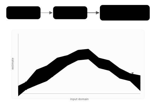
From sparse noisy measurements to a continuous estimate with calibrated uncertainty — the band narrows at observations and widens between them.
Recover latent system states from noisy, indirect, or incomplete measurements while quantifying uncertainty well enough to support decisions.
Methods include Bayesian inference, variational inference, and Markov-chain Monte Carlo (MCMC). These techniques produce calibrated posterior distributions rather than point estimates, enabling risk-aware downstream decisions.
Concrete examples:
- Grey-box identification of building thermal dynamics using SINDYc with MCMC uncertainty quantification — published in Energies (DOI: 10.3390/en13123183), with open-source software on Zenodo.
- Radar-based physiological state estimation (respiration, cardiac motion) as an ongoing adaptive sensing testbed.
See: Prosumer response estimation via SINDYc + MCMC, SINDYc and MCMC framework.
Adaptive decision-making
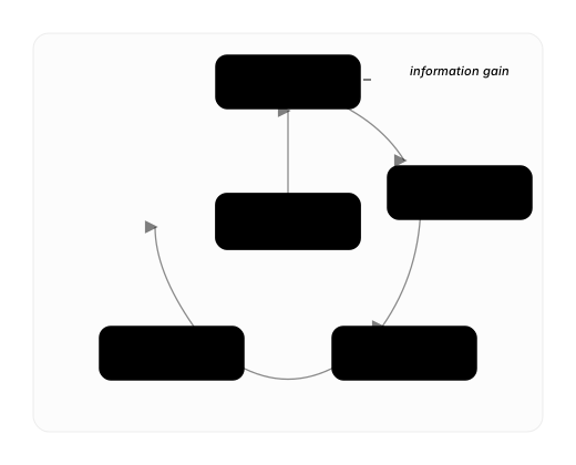
Adaptive decision loop — the next action is chosen to maximize expected information gain given the current belief state.
Use uncertainty estimates and information-gain criteria to choose the next measurement, sensing configuration, experimental condition, or stopping point.
Methods include model predictive control (MPC), optimal experimental design, and information-theoretic acquisition. The same sequential-decision framework that drove target-adjusted MPC for microgrid frequency control now drives adaptive waveform design for biomedical sensing.
Concrete examples:
- Target-adjusted MPC for load frequency control in islanded microgrids with uncertain renewable generation — published in IET Renewable Power Generation (DOI: 10.1049/iet-rpg.2019.0487).
- Adaptive experiment selection for antibacterial combination screening under assay cost and safety constraints (ongoing, manuscript under review).
See: Load frequency control using target-adjusted MPC, AntiSyn-AI for antibacterial discovery.
Closed-loop experimentation
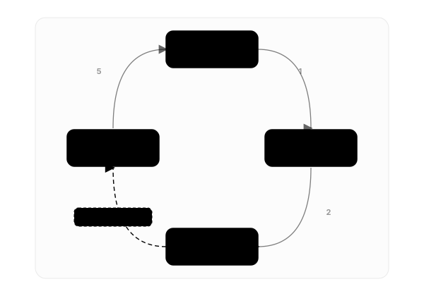
Closed-loop experimentation cycle — measure, infer, decide, act — with an expert review gate before actions that require human supervision.
Connect measurement, inference, and action so systems can adapt data acquisition or experimental plans as evidence accumulates.
This pillar combines sensing, inference, and decision into a feedback loop while preserving human supervision where required. The architecture extends from lab-validated hardware-in-the-loop platforms to human-supervised autonomous bioassay systems.
Concrete examples:
- Three-level hierarchical microgrid control validated on a hardware-in-the-loop laboratory platform — published in Electric Power Systems Research (DOI: 10.1016/j.epsr.2020.106758).
- Human-supervised closed-loop bioassay platform for antibacterial screening (under review).
See: Three-level hierarchical microgrid control.
Mechanistic machine learning
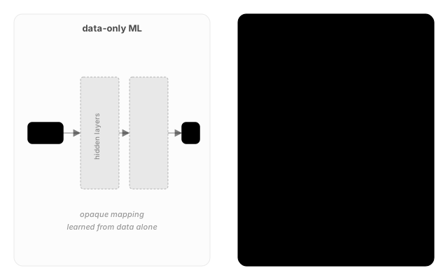
Data-only ML treats the system as a black box; physics-constrained ML embeds known physics (PDE residual) into the learning process.
Combine learned models with physical forward models, scientific priors, and constraints so predictions remain interpretable and actionable.
Rather than treating the system as a black box, we encode known structure — conservation laws, differential equations, sensor models — into the inference or control pipeline. This ensures predictions respect physical feasibility and remain interpretable to domain experts.
Concrete examples:
- SINDYc (Sparse Identification of Nonlinear Dynamics with control) using physical basis functions for prosumer behavior modeling, combined with MCMC for uncertainty quantification.
- Radar forward models for physiological monitoring, encoding electromagnetic propagation physics into the measurement model.
- Modular energy-hub modeling framework encoding thermodynamic and network constraints — GSoC 2016 project, software on GitHub.
See: Modular energy hub framework.
These four pillars apply across all current and prior application domains. See the Research page for the research program overview and the Applications page for where these methods are used.