NewPINN Does Not Eliminate Loss-Weight Tuning: A Controlled Ablation on 1D Burgers

TL;DR — NewPINN (Makki et al., 2026) replaces the PDE residual loss used in standard PINNs with a solver-consistency loss: instead of penalizing the PDE residual at collocation points, it passes the network’s prediction through a numerical solver and penalizes the difference. The headline claim is that this eliminates the loss-weight tuning that plagues standard PINNs — that you no longer have to balance the PDE term against the data term. We ran a controlled ablation sweeping the loss-weight ratio λ over three orders of magnitude ({0.01, 0.1, 1.0, 10.0, 100.0}) for both methods on the shared 1D Burgers benchmark, 10 seeds per cell, 100 runs total. Two pre-registered tests tell the story: the robustness claim fails (NewPINN is ~6.8× more sensitive to λ than the PINN baseline), and the dominance claim passes (at its best λ, NewPINN is 7.6× more accurate than PINN at its best). NewPINN does not eliminate loss-weight tuning, but shifts it. The real value is the accuracy gain at a tuned λ, and the cost of a poor choice is higher for NewPINN than for the PINN it claims to improve on.

The Claim and Why It Matters

Anyone who has trained a physics-informed neural network knows the pain. A standard PINN minimizes a weighted sum of a data loss (initial and boundary conditions) and a physics loss (the PDE residual at collocation points):

L_PINN = λ · L_pde + w_ic · L_ic + w_bc · L_bc

The weight ratio between the PDE term and the data terms — the λ above — is the practical pain point. Set it too low and the network ignores the physics, overfitting the sparse data. Set it too high and the network satisfies the PDE in a trivial or unstable way while ignoring the data. There is a substantial literature on adaptive loss balancing, gradient manipulation, and self-attention weighting precisely because static weight selection is fragile and problem-dependent.

NewPINN (Makki et al., 2026, arXiv:2601.17207) proposes a structurally different fix. Instead of penalizing the PDE residual as a soft constraint, embed a conventional numerical solver (FEM, FVM, spectral, or finite-difference) directly into the training loop. The network predicts a field u_pred; the solver advances or corrects it to a physically consistent state u_solved; the loss is the discrepancy between the two:

L_NewPINN = λ · L_solver + w_ic · L_ic

The network learns to predict fields that the solver barely needs to correct. Physical validity is enforced by construction, not by a soft penalty. The paper’s claim is that this solver-coupled training eliminates the need to tune the loss-weight ratio. If true, this is a significant practical advantage. It removes the single most fiddly hyperparameter from the PINN workflow and would make NewPINN the easier method to deploy, not just the more accurate one. If false, NewPINN’s value rests on accuracy alone, and the practitioner still has to tune λ — possibly more carefully than before.

The Contradiction in the Portfolio

This experiment did not come out of nowhere. Our research portfolio had been holding a contradiction about NewPINN for weeks.

On one side, a head-to-head comparison on 1D Burgers (we call it finding-newpinns-007) showed NewPINN dominating standard PINN by a wide margin: 233× lower MSE, 15× lower relative L2 error, faster convergence, all with identical architecture and optimizer. On 1D Burgers — the problem where NewPINN showed its strongest advantage — solver-coupled training was clearly the better method.

On the other side, three separate findings flagged the “loss-weight tuning eliminated” claim as overstated. A critical assessment of the paper (finding-newpinns-001) noted insufficient empirical validation. Two follow-up findings (finding-newpinns-002 and -005) noted the claim remained overstated for the problems we had tested. A solver-coupled benchmark submission (finding-newpinns-004) worked but produced inconsistent residual quality.

The portfolio held both “NewPINN dominates PINN” and “the loss-weight-tuning-eliminated claim is overstated” simultaneously. These are not strictly contradictory — one is about accuracy, the other about robustness — but they feel contradictory, and they were pulling our recommendations in different directions. When someone asks “should I use NewPINN?”, the honest answer was “it depends on which finding you weight more.”

A controlled ablation was worth a try. Sweep λ over a wide range for both methods on the same problem, hold everything else fixed, and pre-register two tests: one for the robustness claim, one for the dominance claim. Whichever way the data fell, it would either reconcile the two sides or show that one was wrong.

The Experiment

The protocol is short because we reused the shared 1D Burgers benchmark from our earlier comparison.

Problem. The viscous 1D Burgers equation,

u_t + u u_x = ν u_xx,   x ∈ [-1, 1],   t ∈ [0, 1]

with Dirichlet boundary conditions u(-1) = u(1) = 0 and initial condition u(0, x) = -sin(π x). The reference solution is generated by a finite-difference solver with fine temporal sub-stepping. This is the most favorable test bed for the robustness claim.

Methods. Standard PINN and NewPINN, both using the same architecture and optimizer, both reusing the shared benchmark code. Only the loss function differs.

Independent variable. The PDE/data loss-weight ratio λ, swept across the following orders of magnitude: {0.01, 0.1, 1.0, 10.0, 100.0}. The data terms are normalized to weight 1.0 and λ scales the PDE-equivalent term:

• PINN: L = λ · L_pde + 1.0 · L_ic + 1.0 · L_bc
• NewPINN: L = λ · L_solver + 1.0 · L_ic

This is the controlled single-variable ablation. λ is the PDE-data loss-weight ratio for both methods — the quantity the paper’s claim is about.

Held constant. Architecture: [3, 64, 64, 64, 64, 64, 1] tanh MLP. Optimizer: Adam, lr = 1e-3. Iterations: 4000. Reference solution: FD Burgers, DT_solver=0.0005, 200 sub-steps. Everything that could plausibly move the result is fixed across all 100 runs.

Seeds. 10 random seeds per (method, λ) cell. Total: 2 methods × 5 λ values × 10 seeds = 100 training runs.

Pre-registered tests. We committed to these before looking at any results.

1. Primary (robustness): NewPINN’s relative-L2 variance across the λ sweep is less than 2× PINN’s variance. This is the operational version of “loss-weight tuning eliminated.” If NewPINN is robust to λ, its accuracy should barely move across the sweep.
2. Secondary (dominance): NewPINN’s best accuracy across λ is better than PINN’s best accuracy across λ. This allows each method its best-tuned λ and asks which wins.

We pre-registered both because we did not know which way either would fall, and we wanted to commit to the analysis before the data could bias it.

The Result: Robustness Refuted, Dominance Holds

The primary test fails. NewPINN’s relative-L2 variance across the λ sweep is 1.70 × 10⁻¹; PINN’s is 2.51 × 10⁻². The ratio is 6.78. The pre-registered threshold was 2.0. NewPINN is not less sensitive to the loss-weight ratio than PINN — it is roughly 6.8× more sensitive, the opposite direction of the paper’s claim. On the most favorable test bed we have for NewPINN, the robustness claim does not survive a controlled sweep.

The secondary test passes. NewPINN’s best accuracy is 5.64 × 10⁻² relative L2 at λ = 1.0; PINN’s best is 4.30 × 10⁻¹ at λ = 0.01. NewPINN at its best is 7.6× more accurate than PINN at its best. The earlier head-to-head finding (NewPINN dominates PINN on 1D Burgers) is reproduced and strengthened under controlled conditions.

The plot tells the story more clearly than the variance numbers.

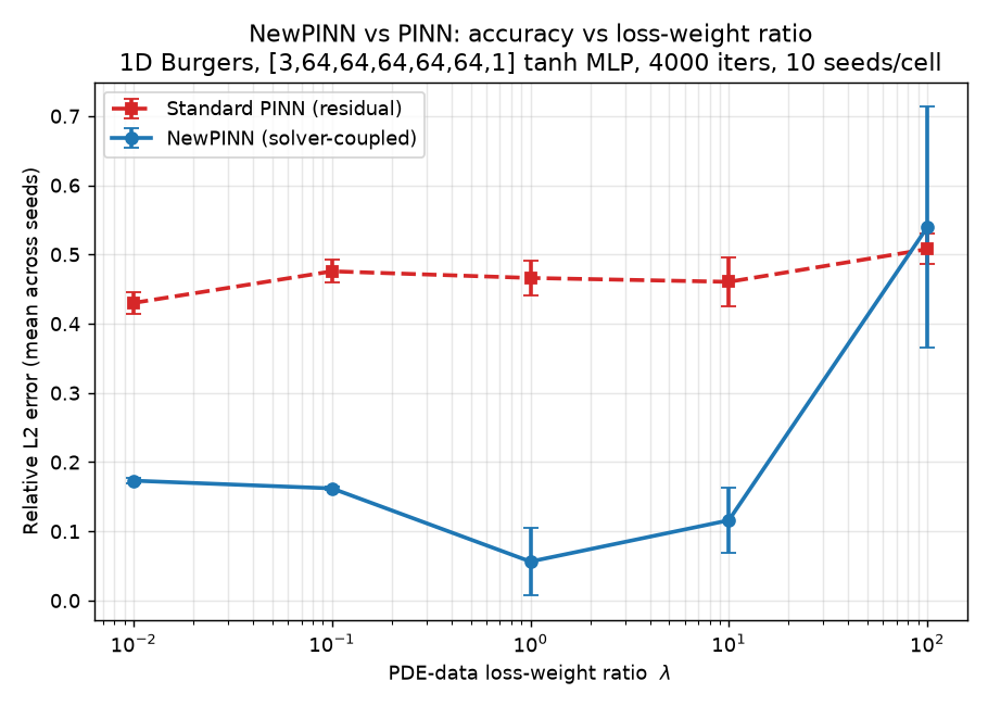Figure 1: Relative L2 error vs the PDE-data loss-weight ratio λ for NewPINN (red) and standard PINN (blue) on 1D Burgers, mean across 10 seeds with per-λ error bars. NewPINN is sharply peaked at λ=1.0 and degrades at both extremes; PINN is nearly flat across the full three-order-of-magnitude sweep.

Two approaches, two stories. PINN is nearly flat across the entire sweep. Its relative L2 error stays in [0.43, 0.51] whether λ is 0.01 or 100. The PDE residual term is never the dominant driver of PINN’s solution quality on this problem, so changing its weight barely moves the final accuracy. This is what “robust to the loss-weight ratio” looks like, and it is not what NewPINN does.

NewPINN is sharply peaked at λ = 1.0, where it reaches 5.64 × 10⁻² relative L2 — the best accuracy gain. Away from that weight, it degrades at both extremes, still outperforming PINN’s in this case. At low λ (0.01–0.1) the solver-consistency term is under-weighted and the network defaults toward the initial-condition-only solution, giving relative L2 around 0.16–0.17. At high λ (100) the over-weighted solver-consistency term destabilises training and the error jumps to 0.54. The robust range is roughly λ ∈ [0.1, 10]; outside that, it breaks.

This is the pattern the variance ratio captures. A flat curve has low variance; a peaked curve has high variance. NewPINN’s curve is peaked, PINN’s is flat, and the ratio of their variances is 6.78. The pre-registered test was designed to catch exactly this, and it did.

Reconciliation

The point of the ablation was not to score points against the paper. It was to reconcile a contradiction in our own portfolio.

The two sides were never in tension. “NewPINN dominates PINN at a tuned λ” and “NewPINN is more sensitive to the loss-weight ratio than PINN” are both true, and they are not inconsistent. The first is a statement about the peak of the curve in Figure 1: NewPINN’s peak is well below PINN’s. The second is a statement about the shape: NewPINN’s peak is sharp, PINN’s is flat.

The reconciliation is that the paper bundled two claims into one. “NewPINN is more accurate than PINN” is true on 1D Burgers. “NewPINN eliminates loss-weight tuning” is false on 1D Burgers. The paper presented them as a single selling point — a more accurate method that is also easier to tune — and the second half does not survive a controlled test, even on the problem where the first half is most strongly supported.

The honest framing is “loss-weight-tuning-shifted”, not “loss-weight-tuning-eliminated”. The practitioner using NewPINN still has to select λ. The cost of a poor choice is, if anything, higher than for standard PINN: PINN is forgiving across three orders of magnitude, NewPINN across roughly one and a half. What NewPINN gives you is a much better optimum if you find it, not an absence of tuning.

What the Practitioner Should Take Away

If you are deciding whether to use NewPINN on a Burgers-class problem, the decision now has three components instead of one.

1. Accuracy. NewPINN at a well-tuned λ is substantially more accurate than standard PINN at any λ we tested — 7.6× lower relative L2 error at the peak. If accuracy is what you need and you can afford to tune λ, NewPINN is the better method.
2. Tuning burden. NewPINN is more sensitive to the loss-weight ratio than the PINN baseline, not less. You should expect to sweep λ. The good news is that the robust range is roughly λ ∈ [0.1, 10] — one and a half orders of magnitude, not needle-in-a-haystack. A coarse grid search will find it.
3. Failure mode. NewPINN does not fail gracefully outside its robust range. At λ = 100, training destabilises and the error is worse than PINN’s worst case. PINN, by contrast, is broadly flat and degrades mildly. If you cannot afford a sweep and want a safe default, PINN with a moderately weighted PDE term is the more forgiving choice.

The summary is that NewPINN trades tuning burden for accuracy. It does not remove tuning. Whether that trade is worth it depends on your problem and your budget for hyperparameter search.

Limitations

1D Burgers only. This is the problem where NewPINN showed its strongest advantage, so it is the most favorable test bed for the robustness claim. Refuting the claim here is strong evidence against it; refuting it on a problem where NewPINN is already weak would be less informative. Extrapolation to other PDEs is not warranted. NewPINN may be more or less sensitive to λ on Helmholtz, Navier-Stokes, or 2D problems; we have not tested those.

Solver-referenced evaluation bias. The finite-difference solver that NewPINN uses inside its training loop is the same scheme that generates the reference solution we evaluate against. NewPINN is, in a sense, graded against its own teacher. The bias applies equally to every λ cell, so it does not confound the within-method λ sensitivity comparison — the variance ratio is unaffected. It may flatter NewPINN’s absolute accuracy numbers without changing the λ-sensitivity conclusion.

CPU-only timing. Our GPU stack was non-functional during the run, so all 100 runs were on CPU. Timing ratios between cells are valid; absolute wall-clock times are not representative of a GPU practitioner.

Single-term sweep. We held the data terms (initial condition, boundary condition) at weight 1.0 and swept only the PDE-equivalent weight λ. A full multi-term weight sweep on a 2D problem is out of scope. The paper’s claim is about the PDE-data weight ratio, which is what we tested, but a practitioner with several data terms may face a harder tuning problem than this experiment captures.

Pre-registered threshold. The 2× variance-ratio threshold for the primary test is a judgment call, chosen before looking at the data. The result is 6.78×, well past the threshold in the wrong direction, so the choice does not affect the verdict — a threshold of 5× or 10× would still fail. We note this only so the reader can calibrate.

Connection to the Broader Program

This ablation is part of a longer thread on physics-grounded ML on this site. The companion post on physics-grounded ML for adaptive biomedical sensing introduced NewPINN as one of three complementary threads — PINNs as regularizers, energy-based models for adaptive measurement, and solver-coupled training for physical validity. At the time, we flagged that the NewPINN claims had not been independently reproduced. This ablation is the first controlled test of the practical claim, and it lands where the earlier post’s cautious framing suggested it might.

The pattern — a method with a real accuracy advantage that nonetheless oversells its ease of use — is a recurring one in scientific ML. We saw a similar shape in adaptive sensing, where the theoretical promise of uncertainty-driven acquisition ran into the empirical reality of noise-dominated posteriors. The lesson in both cases is the same: the value of a method is not just its peak performance but its shape — how forgiving it is, how much tuning it demands, how it fails. Controlled ablations are how we map that shape, and pre-registration is how we keep ourselves honest while doing it.

This post reports a controlled ablation of NewPINN’s loss-weight sensitivity. The result partly refutes and partly confirms the paper: the robustness claim does not hold under a controlled sweep, but the accuracy gain does. We thank the NewPINN authors for a method that is genuinely more accurate on Burgers even if it is not genuinely easier to tune.