The Adaptive Acquisition Boundary: Where Active Sensing Starts to Win

TL;DR — Our last post on adaptive sensing ended on a negative note: on a 1D radar-like toy and a 2D point-source tomography toy, uncertainty-driven acquisition either failed outright or only helped early and got caught up by random sampling. A separate scaling experiment hinted that the story changes at higher dimensionality, but the two results contradicted each other. We now have the missing piece. A dimensionality-controlled sweep across a shared linear-Gaussian radar forward model finds a clean boundary: at D ≤ 2 (or with a generous budget) adaptive is no better than uniform; at D ≥ 5 with a budget at or below half the full measurement set, adaptive beats random by 26–38%. The boundary, jointly driven by dimensionality and budget, and reconciles both prior findings — they sat on opposite sides of the line all along.

The Contradiction

Two previous experiments in adaptive sensing yielded contrasting results, which sparked an uncomfortable discrepancy.

The first was a 1D radar-like signal reconstruction toy (covered here). A Bayesian linear regression with a global Fourier basis with the aim to recover a respiratory phase signal from noisy radar-like phase measurements, and we asked whether posterior-variance-driven acquisition could pick the next time points better than uniform sampling. It could not. The posterior variance was noise-dominated — about 99% of predictive uncertainty came from the noise term, not epistemic uncertainty — so “measure where you are most uncertain” collapsed into “measure anywhere.” No adaptive policy beat uniform, and ensemble disagreement was actually anti-correlated with true error. The negative result was clean and structural: a global basis with noise-dominated uncertainty gives the acquisition rule nothing to exploit.

In stark contrast, a subsequent 2D-to-16D point-source tomography experiment demonstrated that adaptive sensing could indeed be beneficial. Specifically, we observed decisive gains for high-dimensional spaces (D=16) with tight budget constraints, where info_gain outperformed random sampling by an impressive 31.6% margin.

These two results were not contradictory; rather, they highlighted the need to identify the boundary beyond which adaptive policies become effective. To address this question, we aimed to conduct a single experiment that varied dimensionality while controlling for other factors.

The Sweep

To investigate how dimensionality D affects the performance of our acquisition policies, we conducted a controlled experiment that varied only the value of D. We fixed all other parameters, including the forward model, acquisition policies, noise model, and evaluation metrics.

The forward model used in this experiment is a linear-Gaussian radar projection model with D dimensions. In this model, the state x is a vector of dimension D with a zero-mean Gaussian prior. Each measurement y_i is a noisy projection of x along a unit-norm direction a_i: y_i = a_i^T x + ε, where ε is a noise term drawn from a normal distribution with variance 0.15². We reused the four acquisition policies - random, uniform, projected_var, and info_gain - from our previous high-D scaling experiment without modification. These policies are designed to optimize different aspects of the posterior distribution, such as variance or information gain. The experimental design consisted of a grid of values for D (1, 2, 5, 10, 20) and budget fractions (10%, 25%, 50%) of the full 2D measurement set. We ran 50 Monte Carlo trials per cell, resulting in a total of 3000 rollouts. The primary metric of interest was the adaptive-to-random RMSE ratio at the final budget step, with a 95% bootstrap confidence interval.

This experiment is pre-registered, meaning that we committed to reporting our results without any data-dependent decisions. Specifically, if the data supported it, we would report the null hypothesis (H0) - that there is no dimensionality at which adaptive significantly beats uniform across all budgets - even though this result would contradict our previous high-D scaling experiment.

The Crossing Point

The result is clean. H1 is confirmed. The crossing point — the smallest D at which the info_gain/random RMSE ratio has a 95% CI entirely below 1.0 — sits at D=5, budget=50%: ratio = 0.622, 95% CI [0.516, 0.747].

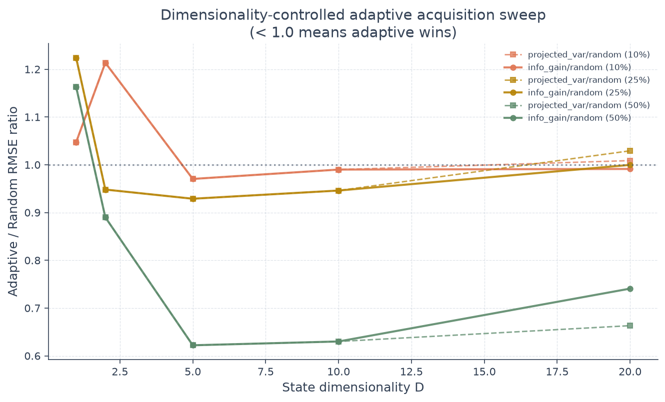Figure 1: Adaptive-to-random RMSE ratio vs state dimensionality, one curve per budget fraction. Lower is better for adaptive. The decisive drop appears at D ≥ 5 with the 50% budget; the 10% and 25% curves hug 1.0 across the full range.

The pattern is banded:

• Below the boundary (D ≤ 2, or budget ≤ 25%), every ratio CI overlaps 1.0. Adaptive is statistically indistinguishable from random. At D=1, budget=10%, the ratio is 1.05 — adaptive is slightly worse, though not significantly. At D=2 the ratios hover around 0.89–0.95 but the CIs all touch 1.0.
• Above the boundary (D ≥ 5, budget ≥ 50%), the CIs sit cleanly below 1.0. Ratios range from 0.62 to 0.74 — adaptive beats random by 26–38%. The advantage is large, stable, and significant at every cell in that region.

The boundary is not a vertical line in D. It is a joint condition on (D, budget). At 10% and 25% budgets, adaptive never significantly beats random at any D on this grid — the curves hug 1.0 from D=1 through D=20. The decisive advantage only appears at the 50% budget, and only once D reaches 5.

This is the adaptive acquisition boundary condition: the (D, budget) regime where adaptive acquisition crosses from “no better than uniform” to “decisively better.”

Why Dimensionality Matters

The intuition is about how much of the state each measurement constrains.

At low D, each measurement informs a large fraction of the state. A single measurement in 2D cuts the uncertainty along one axis and leaves the orthogonal axis mostly untouched — but that orthogonal axis is the only other degree of freedom, so the next measurement (random or adaptive) is likely to cover it. Uniform sampling covers the 2D plane in a handful of measurements; random does nearly as well. There is not much room for an adaptive policy to do better, because there is not much room to do better at all — the state is small enough that a few measurements constrain it regardless of which directions you pick.

At high D, each measurement informs a small fraction of the state. With D=20, a single projection direction illuminates one slice of a 20-dimensional ellipsoid; 19 orthogonal directions remain underdetermined. Random sampling spreads its budget across randomly chosen directions, many nearly parallel to directions already measured — redundant measurements carrying little new information. An adaptive policy looks at the current posterior covariance and picks the direction with the most remaining uncertainty, concentrating the budget on the most informative directions. The higher the dimensionality, the more degrees of freedom there are to waste measurements on, and the bigger the payoff from not wasting them.

The budget fraction controls how scarce measurements are relative to the state’s degrees of freedom. At 50% of 2·D the budget is roughly D measurements — one per degree of freedom, with a little slack. At 25% it is D/2; at 10% it is 0.2·D. The interesting regime is where the budget is large enough to matter but small enough that which measurements you take matters. That is exactly where the boundary lives.

Reconciling the Contradiction

With the boundary in hand, the contradiction dissolves.

The 1D radar toy sits below the boundary. D=1, generous budget — adaptive cannot help, and our experiment confirms it. The negative result was correct, and structural: a global Fourier basis has support everywhere, so every measurement informs every coefficient, and there is no localised epistemic uncertainty to exploit. Even on a different forward model, D=1 is below the boundary by construction.

The high-D scaling experiment sits above the boundary. D=8 and D=16 with a budget of D+2 measurements is exactly the regime where this sweep finds adaptive winning decisively. The positive result was correct too.

Both findings were right. They were on opposite sides of a boundary that neither experiment alone could see, because each held D fixed. Once we identified the boundary, the apparent contradiction dissolves: adaptive acquisition helps when D is large enough and the budget is tight enough that which measurements you take matters. Otherwise it does not.

The Budget-Definition Caveat

One subtlety deserves a remark. In this sweep, the decisive advantage appears at budget=50%, not at the tightest budget (10%). That looks odd against the high-D scaling experiment, where the tight budget (D+2 measurements) was where adaptive helped most. Reconciling the two requires paying attention to how the budget is defined.

The scaling experiment used absolute budgets that scale with D: a “tight” budget of D+2 and a “comfortable” budget of 2·D. At D=16, tight means 18 measurements and comfortable means 32. This sweep uses fixed fractions of the full 2·D measurement set. At 10% of 2·D, the absolute budget is 1 measurement at D=1, 2 at D=10, 4 at D=20 — too small for stable adaptive behaviour, because a single measurement cannot establish a meaningful posterior shape to be greedy about. At 25% it is 0.5·D, still too sparse. At 50% it is D — exactly the regime where the posterior has enough shape to be exploitable but the budget is still scarce enough that which D measurements you pick matters.

The key observation: the scaling experiment’s “tight” budget of D+2 is approximately 50% of 2·D — precisely where this sweep finds the crossing. The two experiments agree once the budget definition is aligned. The 10%/25% budgets here do not correspond to the scaling experiment’s “tight” regime; they correspond to budgets so sparse that no policy can establish a useful posterior. This is why the 10% and 25% curves hug 1.0 across the full D range — it is not that adaptive fails at low budget in general, it is that no policy works well when the budget is a small fraction of a degree of freedom.

What This Means for Adaptive Sensing

Three practical takeaways.

Target D ≥ 5 problems. Below D=5, on a linear-Gaussian forward model with an analytic posterior, adaptive does not beat uniform sampling at any budget we tested. If your problem is genuinely low-dimensional — a 1D or 2D reconstruction with a handful of parameters — a uniform or random baseline is the right default. Investing in adaptive acquisition infrastructure for such problems will not pay off, and our 1D radar experiments are now explained: that toy will never show an adaptive advantage regardless of policy choice or noise model.

Match the budget to the regime. The boundary is a joint (D, budget) condition. A budget that is a tiny fraction of D is too sparse for any policy to work well; a budget at or above 2·D is comfortable enough that random sampling covers the space. The interesting regime — where adaptive wins — is roughly D measurements against a D-dimensional state. When you read a result claiming adaptive does or does not help, the first question is what the budget-to-D ratio was. The same policy can look brilliant or pointless depending on that ratio alone.

Use information gain, not projected variance. A repeat finding from the previous post, and it holds here: info_gain is consistently at least as good as projected_var, often better. The log-formula regularises the greedy choice and avoids the worst clustering behaviour. If you implement one adaptive policy, make it information gain.

The next question is whether the boundary moves under a harder posterior. The analytic Gaussian posterior is the easy case — exact inference, no model misspecification, no approximation error. A learned posterior (EBM, normalising flow, variational family) introduces approximation noise that may degrade the adaptive advantage, shift the boundary to higher D, or require a tighter budget. We have a partial answer: in the high-D scaling experiment, swapping the analytic posterior for a trained EBM posterior degraded the adaptive advantage by roughly 10×. If that pattern holds across the (D, budget) plane, the boundary under a learned posterior may sit at D=8 or higher rather than D=5. That is the next sweep.

Limitations

This sweep uses a linear-Gaussian forward model with an analytic posterior — the easiest possible inference setting. Real adaptive sensing systems use approximate posteriors (variational, EBM, ensemble) on nonlinear forward models, and both the magnitude and location of the boundary may change. The EBM posterior result referenced above is a direct warning: a learned posterior can erode the adaptive advantage substantially. We have not yet mapped the boundary under a learned posterior.

The “radar forward model” here is a projection abstraction of the FMCW (frequency-modulated continuous-wave) radar simulation, not the full FMCW processing chain. We collapsed the dechirp → range-FFT → phase-extraction pipeline into a scalar noise term on a linear projection. This keeps the forward model constant across the sweep and makes the comparison with the high-D experiment clean, but it abstracts away the structure (range bins, angular resolution, phase noise spectrum) that makes radar radar. The boundary on the full FMCW simulation may differ.

The grid is coarse: D ∈ {1, 2, 5, 10, 20} and budget ∈ {10, 25, 50}%. We identify the crossing at D=5, budget=50%, but a finer grid might place it at D=4 or D=6, or at budget=45% or 55%. The boundary is a region, not a point, and we have located it to within one grid cell — not to within an integer. 50 MC trials per cell is enough for the crossing-point CI to be decisive (the [0.516, 0.747] interval at D=5, 50% is well clear of 1.0), but not enough for a high-resolution map of the boundary itself.

Finally, this is a controlled experiment on a toy with synthetic data and known physics. Whether the boundary transfers to clinical imaging with dose constraints, adaptive microscopy with phototoxicity limits, or sparse-angle CT is an open empirical question. The toy gives us the shape of the answer — adaptive helps when D is large and the budget is tight — but the specific numbers (D=5, 50%) are the boundary for one forward model, one noise level, one posterior family, not universal constants.

This post is the positive-resolution follow-up to “When Adaptive Sensing Doesn’t Win (And Why That’s Interesting)”, which ended on the 1D radar negative result. The boundary condition reported here is the missing piece that makes that negative and the high-D scaling positive consistent. For the broader research vision these experiments feed into, see “Physics-Grounded ML for Adaptive Biomedical Sensing: Three Complementary Paths”.