When the Schedule Meets the Grid: Three-Level Microgrid Control in the Laboratory
TL;DR — A cost-optimal microgrid schedule can become inappropriate as soon as grid frequency moves. Our three-level architecture coupled a 15-minute energy-management plan to an MPC frequency controller executing every 300 milliseconds, with local controllers tracking the resulting setpoints. Laboratory experiments showed how one tuning weight decides whether a hydro plant follows its economic schedule or departs from it to support frequency.
One asset, two legitimate instructions
Consider a small hydro plant inside a grid-connected microgrid. An energy-management system has scheduled its output to minimise operating cost and power exchange with the utility grid. A few moments later, measured grid frequency falls.
The plant now receives two legitimate but competing instructions:
- stay near the economically optimal schedule;
- increase production to help counter the frequency deviation.
Neither objective can simply replace the other. A controller concerned only with cost may ignore a fast system need. A frequency controller unconcerned with the schedule may discard the plan that coordinates generation, solar production, loads, and grid exchange.
Our research question was:
How can a microgrid connect long-horizon economic dispatch to fast frequency control and physical plant operation without making one controller solve every timescale at once?
Three levels—but not the usual shorthand
“Primary, secondary, and tertiary control” often refers to a conventional hierarchy of local stabilisation, frequency restoration, and economic dispatch. That is not the most precise description of the architecture implemented in this paper.
The proposed levels were:
- Energy-management system (EMS): dynamic economic dispatch for the next 15 minutes.
- Frequency controller (FC): constrained MPC that adjusts the EMS setpoints using measured frequency.
- Plant-level controllers: classical local controllers that track the active-power setpoints sent from above.
The microgrid operated in grid-connected mode. The frequency controller contributed primary reserve by rescheduling controllable power; the paper did not demonstrate islanded operation or a droop-based voltage-restoration hierarchy.
Level 1: make an economic plan
The upper controller solved a dynamic economic-dispatch problem. Its objective combined:
- the cost of power produced by dispatchable generation; and
- the cost or revenue associated with exchanging power with the utility grid.
The plan had to satisfy the microgrid power balance, generator output and ramp-rate limits, and a demand-response condition: dispatchable loads could move consumption in time, but their total energy over the horizon remained unchanged.
Every 15 minutes, the EMS generated active-power references for the controllable units. These references answered the planning question:
Given the forecasts, prices, and technical limits, how should the microgrid operate economically?
They did not answer what to do about a frequency deviation arriving between planning updates.
Level 2: revise the plan when frequency moves
The frequency controller used a linearised aggregate model based on the swing equation. A Kalman-filter-based observer estimated the system state and an unmeasured residual disturbance from frequency and power measurements.
The MPC then optimised a 20-second prediction horizon while enforcing:
- upper and lower active-power limits;
- rate-of-change limits; and
- different penalties for moving each unit away from its EMS reference.
That final weight is the negotiation mechanism between the two levels. A large reference-deviation penalty tells the FC, “honour the economic schedule closely.” A smaller penalty gives it permission to move the unit more strongly for frequency support.
Level 3: make the setpoints physical
The plant-level controllers did not solve another system-wide optimisation problem. Their role was to track the active-power setpoints issued by the upper layers on the laboratory devices.
Keeping this layer simple separates system-level intent from device-level actuation. The EMS chooses an economical operating point; the FC makes fast corrections; local controllers make the equipment follow.
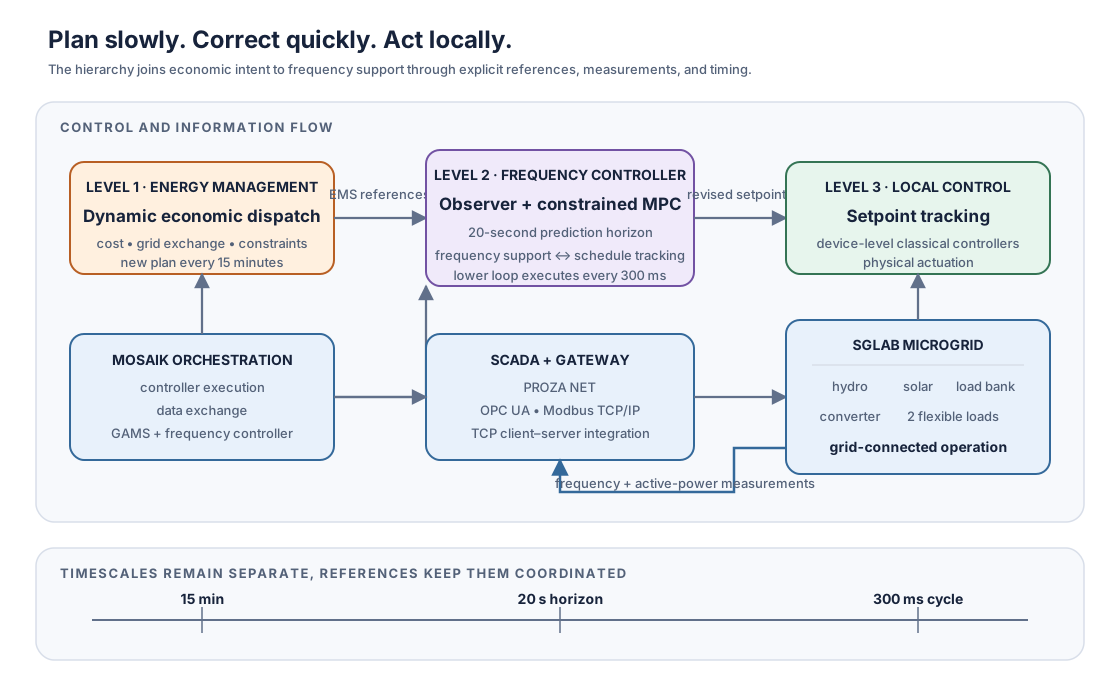
The implemented hierarchy. Every 15 minutes the EMS sends economically optimal active-power references. Every 300 milliseconds the frequency controller combines those references with SCADA measurements and may reschedule the units over a 20-second MPC horizon. Local controllers track the resulting setpoints on the laboratory microgrid.
The integration layer matters
A hierarchy drawn as three boxes is easy. Making independently implemented controllers exchange data at the correct time is the practical challenge.
The laboratory implementation used:
- MOSAIK to orchestrate controller execution and data exchange;
- GAMS to solve the EMS optimisation;
- a frequency-controller implementation connected directly through MOSAIK;
- PROZA NET SCADA to integrate the physical microgrid components; and
- OPC UA, Modbus TCP/IP, and a TCP client–server gateway to connect the control and plant layers.
The operating cycle was explicit:
- every 15 minutes, MOSAIK executed the EMS;
- the EMS setpoints were passed to the frequency controller;
- MOSAIK read frequency and active-power measurements from SCADA;
- the frequency controller calculated revised references;
- those references were returned through SCADA to the local controllers; and
- measurement, optimisation, and actuation at the lower levels repeated every 300 milliseconds.
This co-simulation and SCADA integration—not merely the existence of three control levels—was a central contribution. It allowed different tools and timescales to operate as one closed loop while reusing the laboratory’s existing control infrastructure.
What was in the laboratory
The Smart Grid Laboratory at the University of Zagreb included:
- an 11.8 kW hydro power plant;
- a 10 kW solar plant connected through a three-phase inverter;
- an 8 kW resistive load bank;
- a 20 kW bidirectional AC/DC converter; and
- two controllable 2.4 kW DC electronic loads.
The experiments used this grid-connected laboratory microgrid and its SCADA system. It is therefore more accurate to call the work a laboratory implementation than hardware-in-the-loop: the paper did not connect a controller to a wholly real-time-simulated microgrid.
Two experiments, one revealing weight
Two deterministic experiments demonstrated the hierarchy under different solar-production conditions and different penalties on hydro-plant deviation from the EMS reference.
The hydro plant was the only dispatchable generator. The two controllable loads followed their EMS references closely and did not participate strongly in frequency regulation. The frequency controller could therefore use the hydro unit as its principal reserve provider.
Lower reference penalty
In the first experiment, departure of the hydro plant from its EMS schedule was penalised relatively lightly. At the largest negative frequency deviation, the EMS schedule called for the hydro output to fall—but the FC instead increased it.
This apparent disagreement was the architecture working as intended: the fast controller temporarily prioritised frequency support over the economic reference.
Higher reference penalty
In the second experiment, the hydro reference-deviation penalty was increased. The FC kept the plant closer to its EMS schedule, so the hydro output moved less for frequency regulation.
The comparison makes an abstract tuning parameter tangible:
The reference penalty sets the price, inside the controller, of departing from the economic plan.
It does not determine a universally correct answer. It exposes a policy choice about how much flexibility an asset should provide.
What the paper demonstrated
The work showed that:
- dynamic economic dispatch and fast MPC frequency control could be coordinated in one grid-connected laboratory workflow;
- MOSAIK could orchestrate optimisation, measurement, and SCADA actuation across different timescales;
- the FC could account for constraints and estimated disturbances;
- local loads could stay close to their dispatch schedules while the hydro plant supplied frequency reserve; and
- controller weights could explicitly trade economic-reference tracking against frequency response.
The evidence does not support several broader claims sometimes attached to this work. The experiments did not validate islanded operation, voltage restoration, millisecond inverter droop control, source switching, or a general comparison against simulation-only control.
Limitations
- Grid-connected only. Islanded validation was identified as future work.
- One laboratory topology. The experiments used one hydro unit, one solar plant, and two controllable loads.
- Two deterministic scenarios. They demonstrate functionality, not statistical robustness across operating conditions.
- Plant-level control was not analysed in depth. The paper focused on the EMS and frequency-controller formulations.
- Central orchestration. MOSAIK, the EMS, the FC, and SCADA form a coordinated central architecture with corresponding reliability and cybersecurity considerations.
- Forecast and model dependence. The EMS relies on load and renewable inputs, while the FC uses a linearised aggregate frequency model and approximated disturbance dynamics.
- No controller benchmark. The experiments varied tuning but did not establish superiority over distributed or alternative hierarchical controllers.
The broader lesson
Hierarchical control is often described as decomposition by timescale. The laboratory implementation revealed a second dimension: decomposition by responsibility.
- the EMS owns economic intent;
- the frequency controller owns rapid system support;
- local controllers own physical tracking;
- the orchestration layer owns timing and information flow.
The resulting loop is:
That allocation of responsibility remains relevant far beyond microgrids. Any autonomous experimental or cyber-physical system has to reconcile long-horizon goals with fast feedback and device-level constraints.
For further reading
- Original paper: Beus, Banis, Pandžić, Poulsen, “Three-level hierarchical microgrid control—model development and laboratory implementation,” Electric Power Systems Research, 2020. DOI: 10.1016/j.epsr.2020.106758
- Related project: Three-Level Hierarchical Microgrid Control
- Publication record: Three-level hierarchical microgrid control
- Related controller: Move the Equilibrium, Not the Frequency
- Research trajectory: From Energy Grids to Adaptive Biomedical Sensing